Case Examples of Objectives-Based Site Characterization

This section contains case examples to show how the integrated site characterization (ISC) process can be implemented at various stages of a dense nonaqueous phase liquid (DNAPL) project. The ISC process includes developing objectives, establishing data needs from those objectives, and linking data needs to the selection of characterization tools.

Example 1 – Coal Tar Site in Newark, New Jersey

Current and emerging site characterization tools were selected for a remedial investigation at a former coal tar manufacturing facility in Newark, New Jersey (the site). The purpose of the investigation was to reduce the footprint of an in situ thermal remediation (ISTR) treatment for coal tar DNAPL.

The areas surrounding the site were once flood plains and tidal mudflats along the Passaic River. In the late 1800s, the site and surrounding areas were covered with fill material (historical fill) to allow for development. From approximately that time until May 1983, the site housed various industrial operations involving the production of road tars, phenols, and methyl phenols (cresol and cresylic acid). The site remained vacant from 1986 until approximately 2002, when it was leased as a shipping container storage yard. The site was vacated in early 2012 to allow access for contaminant delineation and to prepare for remediation activities.

Identified contaminants of concern (COCs) from the historical site operations include volatile organic compounds (VOCs), polycyclic aromatic hydrocarbons, phenols, and petroleum hydrocarbons. Contaminants related to the historical fill include semivolatile organic compounds (SVOCs) and metals such as arsenic and lead.

Problem Statement

Uncertainties in the historical conceptual site model (CSM) required a more detailed characterization of the site—in particular, delineating the spatial distribution and estimating the volume and mass of the coal tar DNAPL—to aid in modifying the design of the ISTR.

Uncertainties/Deficiencies with the CSM

The historical CSM for the spatial distribution of DNAPL was based mainly on identifying the areas of the site that were formerly occupied by coal tar production operations. The spatial distribution of DNAPL was unknown within the differing lithological units, but was assumed to be primarily within the historical fill.

Data Collection Objectives and Their Basis

The data collection objectives for the site included the following:

• a detailed lithologic description for the design of the thermal treatment system (vertical)
• a contaminant distribution to design the aerial distribution of thermal treatment (three-dimensional [3D])
• a contaminant mass estimate to design the thermal treatment and duration within each lithology

Data Needs and Gaps

The following data were required to meet the data collection objectives for the thermal treatment remedy:

• the volumes of discrete lithologic units affected by coal tar DNAPL
• the characteristics that differentiate each lithological unit (porosity)
• the DNAPL saturation distribution within each lithological unit
• the properties of the nonaqueous phase liquid (NAPL)
• a contaminant mass estimate to design the thermal treatment and duration within each lithology

Data Resolution

The density of the data collected and the interpolation routine for estimating the extent of the DNAPL distribution were used to select the locations for the thermal treatment wells. The wells were placed on approximately 10 ft centers for the shallow treatment and 20 ft centers for the deep treatment. The density of the data collection varied depending on the historical production practices of each given area (for example, administrative area, lagoon area).

Investigative Tools and Data Collection

A site investigation “toolbox” was used to significantly enhance the ability to characterize the spatial architecture of DNAPL source zones. This toolbox approach provided multiple scales of measurement and data quality, within two main categories of technologies: (1) dense spatial data, often with higher detection limits, and producing qualitative information used to guide the sampling strategy; and (2) compound-specific, generating quantitative, precise data with low detection limits. These two categories of measurement technologies used in tandem produce a more complete and accurate data set, which can further inform the quantification and uncertainty assessment of DNAPL mass. The following site characterization tools were used as part of the remedial investigation:

• cone penetrometer (CPT) friction log on laser induced fluorescence (LIF) tool
• LIF profiles providing semiquantitative response to concentration of coal tar
• sonic percussion coring, core recovery, and logging
• shallow test pit logging
• real-time adaptive site management tools (Sharepoint)
• core subsampling and analysis of VOCs, SVOCs, and extractable petroleum hydrocarbons
• qualitative field methods (visual and enhanced visual)
• physiochemical testing for NAPL density and viscosity (R104)

Data Evaluation and Interpretation

With the site investigation toolbox, an adaptive site characterization can be developed by combining both qualitative and quantitative data sets and incorporating real-time updates. The high-qualitative 3D spatial density of the LIF tool was validated by a limited number of detailed sonic cores, analytical samples, and test pits, and the results of the qualitative and quantitative data correlations were compared. The data from the high-density LIF sampling were communicated to the interpretation team, allowing for real-time revisions to the investigation grid where necessary.

The results of the investigation verified that the DNAPL distribution was localized in the historical site production areas; however, the delineation of the DNAPL indicated a need for thermal treatment of DNAPL at depth, which was not part of the historical CSM. The resulting soil volume requiring treatment, as defined in the updated CSM, was three times lower than the initial estimate.

Example 2 – Dry Cleaner Sites in Indiana

Three former dry cleaner sites located in northern Indiana were investigated using adaptive site management tools that collected real-time data to develop a high-resolution site characterization. Dry cleaner operations began at two of the sites in the 1950s and the third in 1981. All three of the sites were operated as dry cleaners into the 2000s, two as recently as 2008. Between 2004 and 2008, each site was characterized with traditional sampling and off-site analysis. Each site had also been subject to in situ chemical oxidation (ISCO) remediation using a single-event direct injection followed by a later nutrient injection to enhance bioremediation.

Problem Statement

The effectiveness of prior remedial actions at the sites had not been assessed. Although reasonably high-density soil sampling (both horizontal and vertical) had been performed at one of the three sites prior to this investigation, the potential threat to adjacent properties had not been assessed, especially the vapor intrusion pathway. Because the three dry cleaner sites were located within a 5-mile radius of each other, the investigation of the sites was coordinated to allow the sampling and on-site laboratory resources be used most efficiently.

Uncertainties/Deficiencies with the CSM

Post-remediation assessment had been performed at only one of the three sites. The amount and spatial distribution of both separate-phase tetrachloroethylene (PCE) and dissolved-phase PCE and daughter products at each site was unknown. All three dry cleaners were located adjacent to both commercial and residential properties that were at risk from potential vapor intrusion.

Data Collection Objectives and Their Basis

• Describe the lithology at each site to identify storage zones and transport zones for the DNAPL and dissolved-phase plume.
• Map the contaminant distribution in the soil source area, dissolved-phase plume, and vapor phase at adjacent commercial and residential building to assess risk.

Data Needs and Gaps

A site lithology assessment was required to better understand the transport and storage of PCE and daughter products in both the source area and associated plume. The density of soil concentration data in the source areas of two of the three sites were needed to determine whether there was a remaining source to groundwater or soil vapor. The groundwater plumes at all three sites were poorly defined in both the horizontal and vertical dimensions. Potential vapor intrusion from the contamination due to off-site groundwater plume and vapor transport had not been assessed at any of the three sites.

Data Resolution

High-resolution data collection was determined to be necessary to address the uncertainty in the distribution of potential PCE source post-remediation, determine the vertical and aerial extent of the associated groundwater plume, and assess the potential vapor intrusion at adjacent commercial and residential properties. Real-time data collection was selected as the best approach to manage placement of sampling locations and vertical resolutions for each phase investigated. Using real-time data to support selection of sampling locations increases the efficiency of resource allocation, significantly reducing the uncertainty of the resulting CSM due to subsurface heterogeneity.

Investigative Tools and Data Collection

To maximize efficiencies, the United States Environmental Protection Agency’s (USEPA) Triad approach was used with a dynamic work plan and on-site real-time analysis for PCE and daughter products at all three sites in one deployment. The project required direct-push technology (DPT) sampling using two rigs for soil, groundwater, and soil vapor. Field analysis was performed at the on-site mobile laboratory, with direct sampling ion trap mass spectrometry using USEPA Method 8265. A limited number of samples for all matrices was collected for off-site laboratory analysis to inform risked-based remedial decision making.

The project involved 15 days of fieldwork—including sampling at the three sites in all three phases (soil, groundwater, and soil vapor) and on-site analysis. Contamination of the soil, groundwater, and soil vapor was assessed by collecting and performing on-site analysis of 640 discrete samples from 172 plan view locations, averaging 64 analyses per day (see Table B-2 below). The actual field execution was completed in 10 days, covering characterization in the soil source areas, associated groundwater plumes, and potential vapor intrusion pathways.

Data Evaluation and Interpretation

When collecting high-resolution data sets, it is important to manage them in real time so the extracted information can support on-site decision making and the data can be communicated effectively to off-site stakeholders and decision makers. A high-resolution site characterization project requires development of a data management and communication plan.

Before any on-site field activities were conducted, the initial CSM for each of the three sites was constructed based on all data available from the previous investigations. All previous contaminant, geologic, and hydrogeologic data were organized into tables and maps. During field execution, the project manager received the data in real time to further direct field operations. This was accomplished with various communications approaches, depending on the location of the project manager (on site or at the office). Hard-copy data of analytical results were provided, often plan view location by plan view location, when the project manager was present on site. When the project manager was not present, the data were transmitted by email. The project manager provided two-dimensional maps to the field crews, often with multiple revisions each day, to assist in the location of future sampling locations. Thus, the project manager was able to determine where data gaps relative to project data quality objectives still existed and to direct resources to fill those gaps.

Final data presentation was in the form of maps, tables, and verbal interpretation in a site characterization report submitted to the Indiana Department of Environmental Management, as required by regulation. The report included all field data, as well as a limited number of off-site fixed laboratory analyses for soil, groundwater, and soil vapor from samples collected concurrently with the samples collected for on-site analysis.

The high level of interaction of the project manager with the field staff is a primary reason the project was able to be executed within significantly less time than allotted. In addition, the project was completed significantly faster than planned because the project team—including the drilling crew, on-site laboratory, and consulting project staff—had executed similar dry cleaner site characterizations using the same approach.

Example 3 – Reese Air Force Base

Beneath the former Reese Air Force Base (AFB) in north Texas is a typical, large, diffuse trichloroethylene (TCE) plume that illustrates the investigative and remedial challenges of achieving USEPA Maximum Contaminant Levels (MCLs). From 1941 to 1997, the site served as a training facility for pilots, and the operations included aircraft maintenance to clean engine parts using TCE. Spent TCE from these operations leaked from an industrial waste line into the underlying groundwater, forming at its maximum extent a 3 mile by ½ mile diffuse plume in the Ogallala Aquifer. This aquifer is the sole source of water for agriculture and potable use for the surrounding community. Vertically, the hydrostratigraphy consists of three major depositional sequences, 20 ft–30 ft of silt, 30 ft–50 ft of caliche, and 100 ft–130 ft of aquifer material. Generally, the groundwater plume extends from the water table 130 ft below ground surface (bgs) over the full saturated aquifer thickness of 50 ft. The aquifer is composed of a very heterogeneous system of interbedded sediments varying from gravels to clays, deposited by alluvial fans and braided streams.

The TCE remediation goal at Reese AFB was to achieve the MCL of 5 micrograms per liter (µg/L). The performance period during development of the original remedy was estimated to be greater than 30 years. Remediation was initiated in 1997 with groundwater extraction and treatment via air stripping and granular activated carbon, with all treated water injected back into the aquifer. The system gradually expanded as the plume was revealed through investigation and sampling of private wells; by 2004, there were 50 extraction and injection wells, using more than 17 miles of piping to transport and treat over 650 gpm.

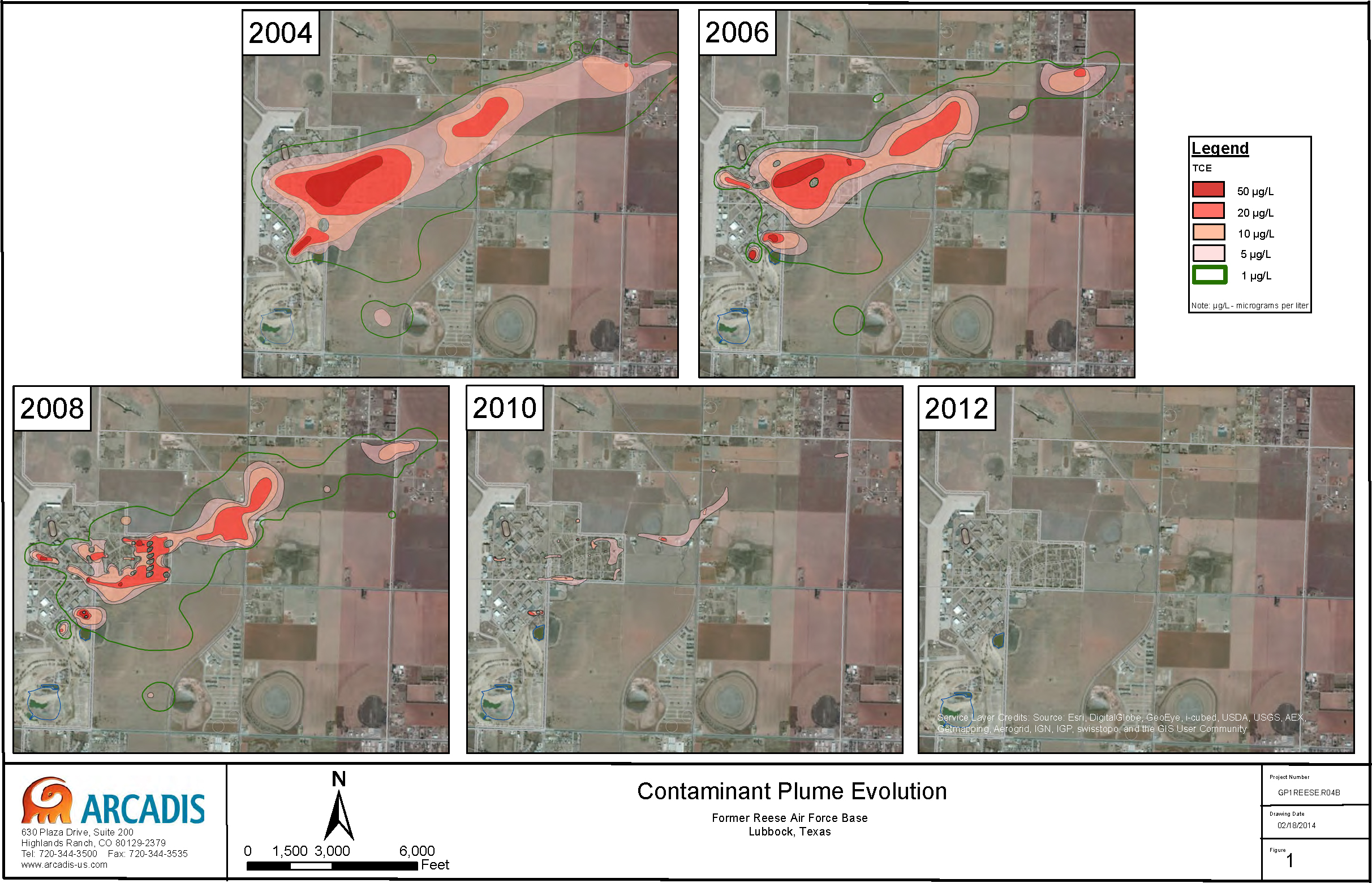
During the first 8 years of operation (1997 through 2004), more than 1.6 billion gallons of groundwater was treated and reinjected at the site; however, the TCE plume showed only limited retreat. In 2004, the site was transitioned to a Performance Based Contract, requiring all monitoring, agricultural, and potable wells affected by the TCE plume to achieve MCLs within 10 years and to maintain those levels for at least 3 years post-treatment monitoring. Figure B-1 shows the TCE plume status at the time of transition to the Performance Based Contract.

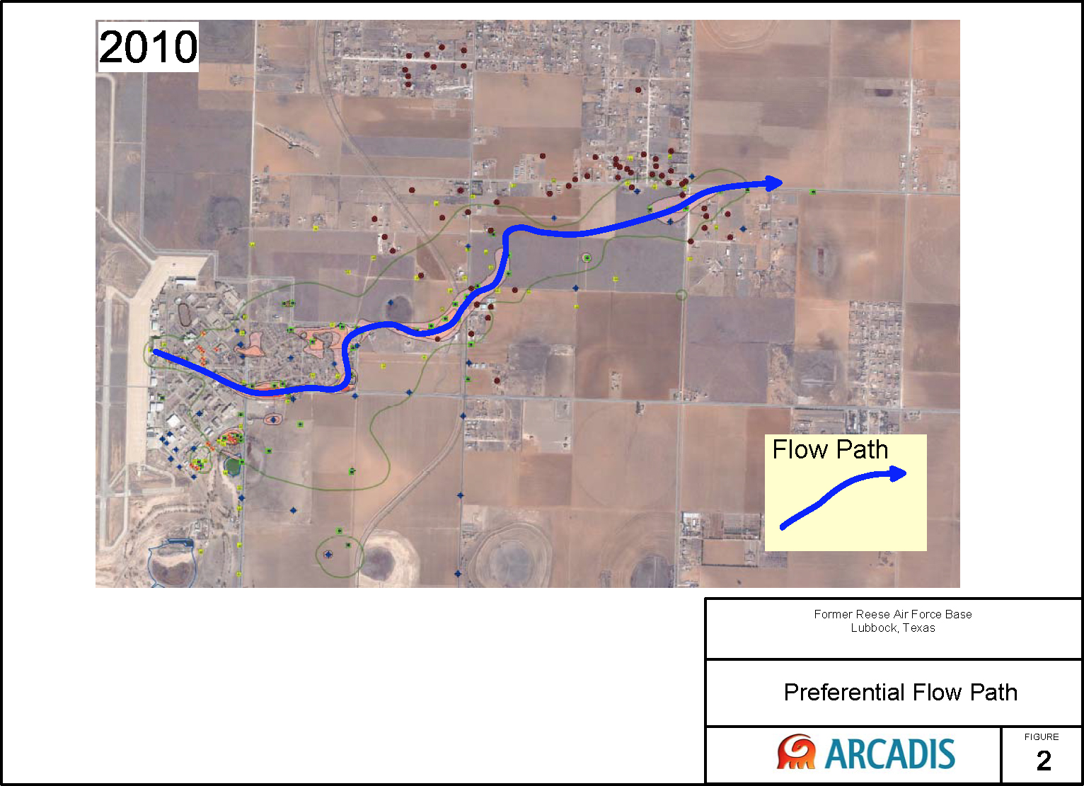
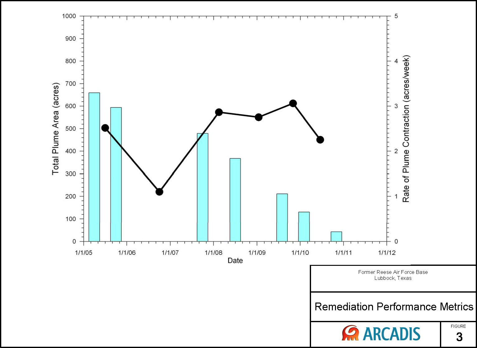
The remedy improvements under the Performance Based Contract accelerated the pace of the remediation, reducing the period of performance by at least 22 years. Figure B-2 shows the TCE plume status in February 2010. Focused groundwater pumping along the core of the plume, combined with strategically directed reinjection of treated groundwater, caused the TCE footprint to contract to a sand-and-gravel channel extending along the axis of the plume. The pace-of-remediation diagram (Figure B-3) shows that the plume footprint has contracted steadily at approximately 3 acres per week. As of 2012, all groundwater concentrations were below the MCL. The total life cycle cost savings achieved through shortening the period of performance is estimated to be greater than $20 M.

Figure B-1. Contaminant plume evolution, Reese Air Force Base, Lubbock, Texas.

Source: Courtesy of Fred Payne, Arcadis.

Figure B-2. The plume's preferential flow path as of February 2010, Reese Air Force Base, Lubbock, Texas.

Source: Courtesy of Fred Payne, Arcadis.

Figure B-3. Pace of remediation, Reese Air Force Base, Lubbock, Texas. The pace of remediation progressed at approximately 3 acres per week.

Source: Courtesy of Fred Payne, Arcadis.

Problem Statement

The problem involved identifying a more effective remedy to shorten the period of performance to less than 10 years and to comply with the pump-and-treat remediation stipulated in the existing Record of Decision (ROD). To achieve site closure within 10 years, the period of active remediation had to be completed within 7 years (allowing for 3 years of post-remediation sampling to confirm remedy completion). The remedial goal was to restore the aquifer to unrestricted potable use by reducing groundwater concentrations for all COCs to less than the MCLs.

The site hydrogeology significantly hindered the remediation effort, with the aquifer structure creating a complex pattern of mass discharge downgradient from the source zone. Thus, the strategy was revised to emphasize the influence of aquifer structure on plume movement, the benefits of pumping and injecting water in targeted locations where remedial performance had slowed, and the use of in situ biological treatment in former source areas to degrade TCE.

Uncertainties and Deficiencies with the CSM

The aquifer structure results in a very complex pattern of mass flux laterally and vertically downgradient from the source. The existing monitoring well network was effective at quantifying groundwater concentrations and identifying potential risks; however, the long well screens provided limited information on detailed plume structure. The initial phase of the project required reassessment of groundwater concentrations using all available data. This included a site-wide synoptic data set collected from all of the investigation wells (>500 wells) and remediation wells (~50 wells), as well as grab samples from more than 100 private irrigation and supply wells within and adjacent to the plume. The revised plume map revealed the following significant findings:

• The contaminant distribution and its movement were highly structured.
• A significant volume of the aquifer previously identified as contaminated was clean.

A review of the CSM and revised plume assessment identified the following inconsistencies:

• Large-scale depositional changes could be identified along the length of the plume.
• Aquifer anisotropy caused a 30-degree deviation between contaminant transport (plume axis) and hydraulic gradient.
• The plume had not invaded the full saturated aquifer thickness in all areas along the plume axis.
• There was no consistent pattern to the plume structure along the plume length—that is, the plume was moving like a ribbon with peak concentrations varying between the bottom, middle, and top of the aquifer, without a discernable pattern.

Data Collection Objectives and Their Basis

The primary data collection objectives were to determine the mass flux along the axis of the plume to better focus remediation efforts. The strategy for optimized site remediation was built around the premise that restoration would accelerate and life cycle costs would decrease if remedy elements were always targeted on the highest mass flux.

Data Needs and Gaps

The strategy required detailed information on the plume and aquifer structure, including the hydrostratigraphy, hydraulic conductivity, groundwater concentrations, hydraulic gradients, and mass flux along and perpendicular to the plume axis.

Data Resolution

Balancing the intermediate scale of depositional features in the aquifer (5 ft–15 ft sequences of sediments), the scale of the remediation (3 miles), and costs to collect data and install remedial systems ($20,000 to $40,000 per soil boring), quality data collected over 10 ft intervals were considered high-resolution information for this site.

Investigative Tools and Data Collection

Soil borings were collected using Rotosonic methods. Grab groundwater and soil samples were collected for each soil boring. Both short- and long-duration aquifer testing were performed to assess aquifer behavior by extracting and injecting water.

Data Evaluation and Interpretation

The CSM was updated based on the groundwater flow and dissolved contaminant transport being focused in the most conductive pathways. This enabled reinterpretation of the composite data from long-screened monitoring wells. Higher groundwater concentrations downgradient of source areas could be used to identify preferred pathways of groundwater and contaminants—that is, the zones with the highest mass flux. The site-wide CSM was subdivided into five smaller units based on variability in groundwater concentrations, age of the plume, accessibility, geology, and local performance metrics. The remedial strategy was recast to match the CSM in each separate sub-unit. This simple strategy, combined with nearly continuous remedy optimization using real-time performance monitoring data, was used to develop remedy enhancements and achieve remedial goals.

Example 4 – Well 12A Superfund Site in Tacoma

The Well 12A site has been designated as Operable Unit 1 (OU1) of the Commencement Bay – South Tacoma Channel Superfund site in Tacoma, Washington (Figure B-4). In 1981, chlorinated solvent, specifically TCE, was detected in groundwater extracted from Well 12A, a municipal water supply well owned and operated by the City of Tacoma Water Department. A ROD-specified air-stripping treatment system developed for Well 12A began operation in July 1983 (USEPA 1983), and based on the findings of a USEPA site investigation, the site was added to the National Priorities List on September 8, 1983.

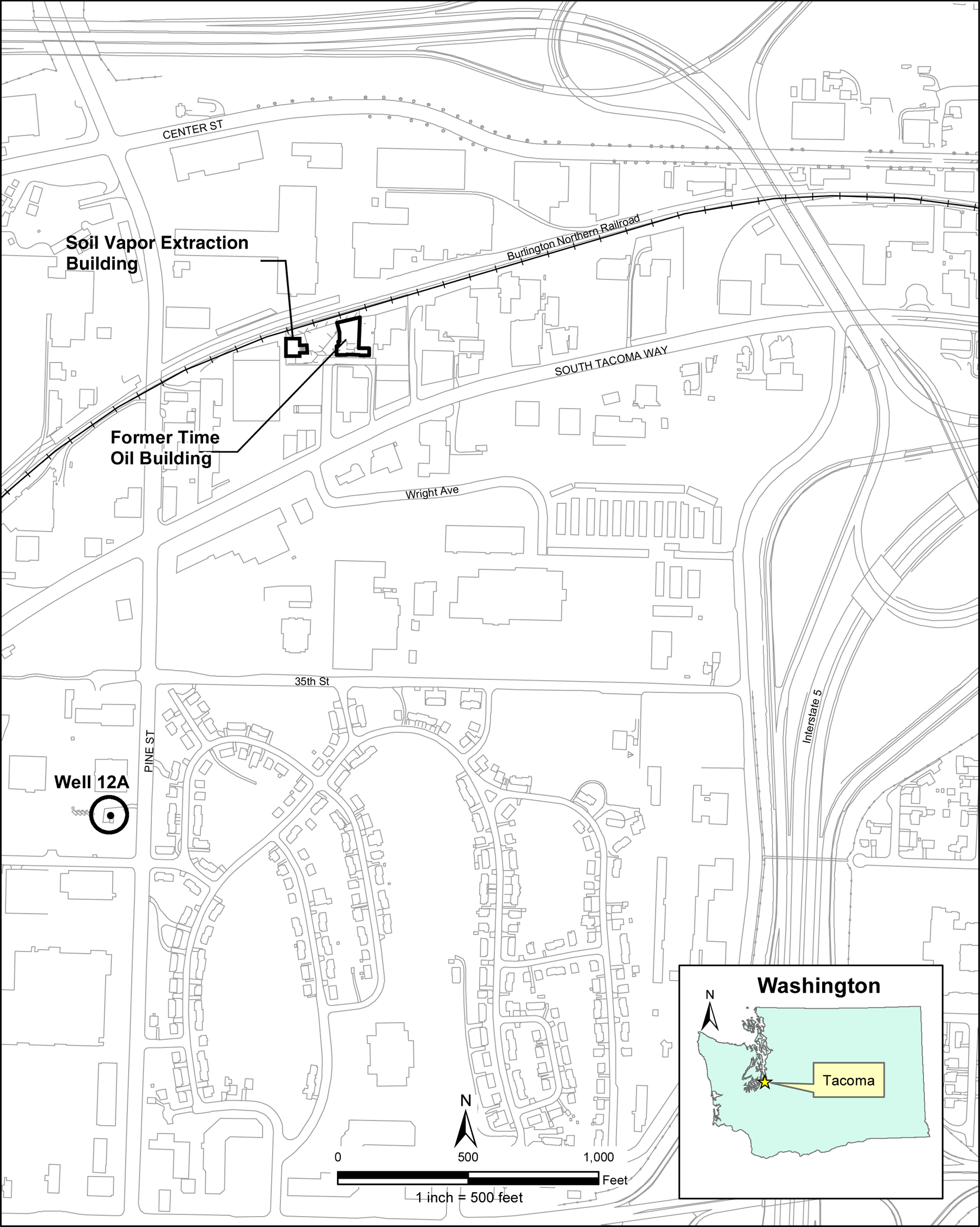
Figure B-4. Well 12A site location map.

Source: Courtesy of CDM Smith.

In early November 1983, Well 12A ceased continuous operations when it was no longer needed for that season. Since then, Well 12A and the treatment system has continued to be used to meet peak summer demand; however, due to the cost of operating the treatment system, use of the well has gradually declined over the years. Well 12A is now typically pumped only during the summer or early fall. However, due to its projected water use, the City seeks restoration of the groundwater to allow for unlimited use of Well 12A.

Further investigation of the TCE contaminant plume identified the primary source of contamination to be the Time Oil Company site. In 1923 or 1924, a paint and lacquer thinner manufacturing facility and an oil recycling facility began operating at the site. The paint and lacquer thinner manufacturing process involved the use of many solvents that were stored on site in barrels, some of which may have leaked. In addition, the process resulted in the formation of a tar-like sludge that was disposed of or stored in various piles on the site. Some of this sludge was also used for fill around the site. These operations continued until 1964 when Time Oil acquired the majority of the property and concentrated on reprocessing waste oil; the waste oil reprocessing continued intermittently until 1976. Following a fire at the facility that destroyed the waste oil processing apparatus in 1976, Time Oil limited operations to the canning of oil, which continued until 1990. Contaminants of concern in groundwater include 1,1,2,2,-tetrachloroethane (PCA), PCE, TCE, cis-dichloroethene (DCE), trans-DCE, and vinyl chloride (VC).

As part of the first ROD Amendment (ROD Amendment #1) (USEPA 1985), 1,200 cy of contaminated soil along a rail spur north of the former Time Oil building was excavated. In addition to the excavation in the railroad spur, contaminated soil was excavated from a narrow strip of land just west of the current soil vapor extraction (SVE) building (Figure B-4). In addition, a groundwater extraction and treatment system (GETS) was constructed and began operation in November 1988 to pump and treat contaminated groundwater near the Time Oil source area. The initial system consisted of a single groundwater extraction well (EW-1); however, in 1995, four additional extraction wells (EW-2 through EW-5), screened at approximately 50 ft–70 ft bgs, were added to the system to improve hydraulic capture and remove more significant quantities of contaminants. Between 1988 and December 2011, the GETS treated over 860 million gallons of groundwater, removing approximately 18,625 pounds of VOCs. In August 1993, an SVE system began operation in the area west of the former Time Oil building where drum storage and disposal operations had previously occurred (also specified in ROD Amendment #1). During construction of the SVE, approximately 5,000 cy of a waste sludge (filter cake) from the oil recycling operations was excavated. Between 1994 and May 1997 (when it was taken out of operation), the SVE removed approximately 54,100 pounds of VOCs. Approximately 25% of the VOCs were chlorinated and the remainder consisted of light-end hydrocarbons.

In 2004 and 2005, USEPA collected soil and groundwater samples from the Well 12A site to assess the effectiveness of the aging GETS. Oily product was identified in some soil samples. In general, groundwater contaminant concentrations had decreased compared to previous samples, but elevated concentrations of chlorinated VOCs were still present.

In September 2008, the third Five-Year Review was completed for the Well 12A site. The report concluded that the existing remedy was not protective, and corrective actions were initiated. In response, USEPA conducted a final Focused Feasibility Study (FFS) to analyze potential remedial alternatives to address ongoing contamination (CDM Smith 2009), and a second ROD Amendment (ROD Amendment #2) was completed in 2009 (USEPA 2009) to address the deficiencies identified in the third Five-Year Review. ROD Amendment #2 updated the remedial action objectives (RAOs) and cleanup goals for the Well 12A site. The amended remedy added excavation and disposal of filter cake and contaminated soils, ISTR, and enhanced anaerobic bioremediation (EAB) as remedial actions for source area treatment. The goals of these additional remediation actions are to (1) address risks from exposure to contaminated soil and groundwater; (2) reduce or eliminate sources of groundwater contamination; (3) reduce the contaminant mass discharge from the source area to the downgradient plume; and (4) prevent further degradation of groundwater quality. The amended remedy included operation of the GETS, as necessary. Between September 2011 and March 2012, a shallow soil excavation was conducted beneath the former east tank farm on the east side of the former Time Oil building. A 14,280-gallon underground storage tank was removed, along with the 6,775 gallons of contaminated liquid and approximately 35 tons of pea gravel from inside the tank. Much of the excavated soil was highly contaminated and required on-site treatment via chemical oxidation prior to off-site disposal. A total of 2,131 tons of contaminated soil was removed during this work.

Implementing the multi-component source treatment required a detailed characterization effort to develop a robust CSM that would support remedial decision making. This effort involved the following:

• Evaluate contaminant mass extents across the source area.
• Map different remediation technologies across the site.
• Develop SMART objectives for individual remediation technologies.
• Evaluate methods for measuring contaminant mass discharge and select one to use for the RAO compliance metric.

The specific activities included (1) performing high-resolution vertical profiling to delineate the vertical and lateral extent of the contaminant source and plume; (2) identifying specific stratigraphic units contributing the highest mass loading (flux) to the downgradient plume; and (3) evaluating methods to measure mass discharge. A 3D visualization model (Mining Visualization Software [MVS™]) was used to define the source and plume boundaries and to evaluate uncertainty.

Problem Statement

Three primary remedial decisions required additional information:

1. Develop and map treatment volumes for ISTR and EAB design within the Time Oil source area.
2. Determine technology-specific SMART objectives.
3. Select the measurement method for evaluating the compliance goal for source treatment, reducing the contaminant mass discharge from the source area to the dissolved plume.

This case study focuses on the data collected in support of decision 1, above, to evaluate the extent of the residual source area, including NAPL extent. The remedial design investigation was designed to meet the following specific primary objectives:

• Collect the data necessary to delineate the horizontal and vertical extent of the soil contamination, including NAPL, beneath and in the vicinity of the former Time Oil building to support delineation of treatment zones for the multi-component remedy.
• Collect the data necessary to evaluate contaminant mass discharge within different areas of the site to evaluate performance of the treatment technologies.

Uncertainties/Deficiencies with the Conceptual Site Model

The investigation activities were also intended to meet the following technology-specific secondary objectives:

• Delineate the distribution of contaminant mass from the Time Oil source area, including areas containing NAPL.
• Delineate the distribution of mass from the Time Oil source area, including areas where secondary sources such as diffused contaminant mass in low-conductivity zones was prevalent.
• Assess vertical variability in specific discharge and mass flux, with the intent to identify vertical depths where the source is contributing the highest mass loading (flux) to the downgradient plume.
• Evaluate if contaminant mass is contained mostly within transmissive zones or mostly within low-permeability zones by comparing the mass flux distribution to the distribution of specific discharge and/or lithology along the transect.
• Determine hydraulic conductivity for stratigraphic units within the VOC plume.

In addition, the following data gaps required additional information to evaluate the mass discharge metrics:

• Determine the hydraulic characteristics of the aquifer.
• Evaluate capture of the source area to evaluate discharge with the GETS extraction system.

Characterization Objectives and Their Basis

The characterization objectives included the following:

• Describe the major stratigraphic units of the upper aquifer containing contaminant mass.
• Quantify the hydraulic properties of the stratigraphic units within the contaminant zone.
• Map the contaminant distribution within the stratigraphic units, including NAPL and soil and groundwater contaminant levels.
• Estimate the contaminant volume and mass.
• Estimate the contaminant mass discharge within stratigraphic units.
• Map the contaminant mass discharge delivered to the GETS extraction wells.

Data Needs and Gaps

The following data needs were identified to achieve the characterization objectives for the source remedy at Well 12A:

• Stratigraphy: Evaluate vertical intervals (elevations) of primary stratigraphic units within contaminant zone at points throughout the Well 12A source area.
• Geologic Properties: Evaluate properties important to design and implementation of treatment technologies and necessary to evaluate contaminant distribution and transport in the subsurface—such as grain size distribution, porosity, and hydraulic conductivity—for each relevant stratigraphic unit within the contaminant zone.
• NAPL Characterization: Delineate the extent of NAPL within each stratigraphic unit.
• Contaminant Extent: Evaluate contaminant levels and extents in soil and groundwater within the Well 12A source area. Evaluate the presence of secondary sources, such as isolated hotspots and/or prevalence of matrix diffusional secondary sources.
• Contaminant Mass Flux and Discharge: Evaluate mass flux and mass discharge at transects near the boundary of the Well 12A source area with sampling for hydraulic conductivity, contaminant concentration, and gradients within stratigraphic layers.
• Source Area Contaminant Mass Discharge: Evaluate capture and contaminant mass discharge of the Well 12A source area using the GETS extraction wells. Evaluate areas where significant mass discharge is occurring (relative to contaminant extents observed in soils and groundwater) to determine the locations for aggressive treatment.

Data Resolution

At Well 12A, 34 soil borings and 12 vertical profile borings were advanced across the source area (Figure B-5). Soil borings were logged continuously using Rotosonic continuous cores. Soil samples were collected based on high-resolution screening with a minimum interval of one sample every 5 ft to 60 ft–95 ft bgs based on results.

Figure B-5. Remedial design investigation and vertical proofing boring locations.

Source: Courtesy of CDM Smith.

Twelve vertical profile borings were advanced every 100 ft along the suspected boundary of the source area. Temporary well screens were initially emplaced every 5 ft from groundwater surface to 95 ft bgs and sampled for contaminant concentrations and slug tested. Sample intervals were reduced to target one sample in each of the five primary stratigraphic units identified. A total of 28 slug tests at eight borings (VP101, VP102, VP103, VP106, VP107, VP108, VP109, and VP112 – see Figure B-5) were performed at various depths to estimate the hydraulic conductivity in the five identified stratigraphic layers (Qva, Qpfc, Qpf, Qpog, and Qpogc). Synoptic groundwater elevations, to assess the horizontal and vertical gradients, were measured at wells screened at discrete depths corresponding to upper (Qva, Qpf, upper Qpfc), medium (Qpfc), and lower (Qpogc) hydrostratigraphic layers of the upper aquifer. The hydraulic conductivity data were used in conjunction with the groundwater sample results and horizontal and vertical hydraulic gradients to calculate the mass flux within each stratigraphic layer.

The GETS pumping tests were conducted by measuring flow rates at the GETS extraction well (EW-1, EW-2, EW-3, EW-5 – see Figure B-6), and at the influent to the treatment system. Pumping tests were conducted at variable pumping rates to evaluate drawdown at monitoring wells; samples were collected for contaminant levels at the extraction wells and/or at the influent to the treatment system, on a daily to biweekly basis until equilibrium was achieved. Flow rates at the extraction well effluents were set at target flow rates for the pumping test, which were as follows:

• EW-1: 80 gpm
• EW-2: 20 gpm
• EW-3: 12 gpm
• EW-5: 7 gpm

Figure B-6. High contamination zone monitoring wells.

For the mass discharge measurement, the target flow rates were chosen to represent a maximum achievable flow rate that sampled the Target Capture Zone–that is, the Well 12A source area. Using particle tracking, it was estimated that, at these flow rates, VOCs concentrations should be representative of the system in approximately 3 months (based on longest travel times from the edge of the Target Capture Zone to the extraction wells). Therefore, the GETS extraction rates determine both the capture zone and the duration of system operation required to obtain integrated measurements of VOC concentrations. To evaluate mass discharge, the integrated VOC concentration measurement from each extraction well or from the treatment system influent was multiplied by the corresponding extraction well or total system discharge, respectively.

Investigative Tools

A total of 34 soil borings were advanced within the known NAPL hotspot and across the downgradient plume based on the results of the screening (Figure B-5). The borings were subject to initial field screening and lithologic logging. Soil cores were field screened for the following:

• ultraviolet (UV) fluorescence – using a Koehler LSI HS-UV-365 lamp
• headspace concentration – using a photoionization detector (PID)
• NAPL – using Cheiron Resources Limited’s (Cheiron) OilScreenSoil field test
• sheen – using visual photologging

Soil samples for laboratory analyses were then collected from the intervals with the highest level of contamination based on the field screening results.

A Geoprobe 8140 track-mounted Rotosonic drill rig and Gus Pech RS 400 truck-mounted Rotosonic drill rig were used to advance 12 soil borings for vertical profiling (Figure B-5). The drill rig advanced a 3.5 inch inner-diameter core barrel ahead of a 4.5 inch outer-diameter casing to collect soil cores. A 6 inch diameter core barrel and 8 inch diameter casing were used to drill to the water table in difficult or gravelly soils. Soil cores were extruded into 5 ft-long plastic bags. The soil cores were logged and screened as described above. The stratigraphic contacts were included in the field logs and used to guide soil sampling and construction of temporary wells for groundwater sampling and slug testing.

After the soil cores were retrieved, a two-jacket drive point screen or Johnson Screen was attached to the core barrel and installed in the boring to create a temporary well for the collection of groundwater samples and slug testing. A Grundfos Rediflo2 2 inch submersible pump was installed into the medium of the drive point screen for groundwater sampling.

In general, one falling head and one rising head slug test were conducted at each location. The slug test data were downloaded from the logger and sent with test information—borehole, screen interval, lithology, water level, and slug dimensions—to a licensed hydrogeologist for data review and analysis. Slug test data were reduced and analyzed following the procedure outlined by Butler (1998) for wells screened below the water table in an unconfined formation.

Data Evaluation and Interpretation

A 3D visualization model was developed using C Tech's MVS™, which incorporates geostatistics. The MVS™ incorporated the site geologic, hydrogeologic and contaminant data into the model. MVS™ provides data interpolation, geostatistical analysis, and 3D visualization tools in a single software system. The following MVS™ integrated geostatistics functions were used for this project:

• Site Evaluation: The MVS™ “Min-Max Plume” technology quantifies the statistical variation in the volume and mass estimates resulting from the current level of characterization. This was used to determine the spatial extent of contamination in soil and groundwater.
• Geology/Stratigraphy: A 3D model of the site geology was created to determine the relationship between the geology and the contaminant plumes. The stratigraphy was updated with the lithologic information contained in the boring logs.
• Analytical Kriging: Interpolation methods were used to accurately determine the minimum and maximum possible plume extents.
• Confidence and Uncertainty Outputs: Areas requiring additional characterization were identified.
• Synoptic Water Levels: Potentiometric contour maps were generated with water level data collected during two synoptic water level measuring events.
• Communication: Visual presentation of the site geology and contamination was critical for effective communication, including the ability to integrate geologic information, environmental contamination data, site buildings, roads, and aerial photographs into a model.

Geology

The Well 12A site is located within the Clover/Chambers Creek Watershed. Stratigraphic interpretation is based on the Draft Geologic Map of the South Tacoma 7.5-minute Quadrangle (Troost 2011). Lithologies of continuous core soil samples collected during investigations were compared to stratigraphic descriptions in the geologic map, and stratigraphic information and interpretation contained within the geologic map were used to refine understanding of the lithostratigraphic units beneath the Well 12A site. The interpreted stratigraphic units include the following (from shallowest to deepest):

• filter cake and artificial fill
• Steilacoom gravel (Qvs), vadose zone
• Vashon till (Qvt), vadose zone
• Vashon advanced outwash deposits (Qva), saturated zone
• coarse-grained deposits of pre-Fraser glaciation age (Qpfc), saturated zone
• sedimentary deposits of pre-Fraser glaciation age, undifferentiated (Qpf), saturated zone
• coarse grained glacial deposits of pre-Olympia age (Qpogc), saturated zone
• till of pre-Olympia age (Qpogt), aquitard

Figure B-7 illustrates the MVS™-modeled geologic kriging and extents of each of these units across the site. Where present, fill material, including filter cake-like material, is generally encountered from ground surface to approximately 1.5 ft–5 ft bgs. The geologic map shows the Well 12A site vicinity as mantled by Qvs. Soils encountered in the uppermost portion of each boring, excluding fill and filter cake material, are consistent with the description of the Qvs unit, consisting primarily of gravelly sand and sandy gravel with varying silt content. The bottom contact with the underlying Qva unit is generally encountered at depths of 25 ft–32 ft bgs.

Figure B-7. 3D visualization of stratigraphic units.

Source: Courtesy of CDM Smith.

Soil characterized as Qva is first encountered at depths of 23 ft–33 ft bgs. The bottom of the Qva unit is at 35 ft–52 ft bgs. Soil characterized as Qva is generally distinctive and consists primarily of poorly graded, medium-grained sand with varying amounts of rounded gravel and lesser amounts of silt. Groundwater is typically encountered within the Qva unit.

A fine-grained silt or clayey silt layer characterized as the Qpf unit is in select areas of the Well 12A site. Where present, it is encountered at depths of 47 ft–52.5 ft bgs and observed to be 1 ft–13 ft thick. There are two noncontiguous occurrences of this unit at slightly different elevations.

The upper occurrence of this unit is generally at elevations greater than 200 ft above mean sea level (amsl), and the second occurrence is found generally below 200 ft amsl. In at least one location (VP109), both occurrences of the silt layer were observed separated by approximately 5 ft of sandy gravel. This suggests that the two separate layers of fine-grained sediment were deposited at different times and are not laterally contiguous across the Well 12A site.

In several of the borings, small wood fragments resembling bamboo shoots and grass were observed within the Qpf unit. The limited aerial extent and lateral discontinuity of the unit across the Well 12A site, combined with the presence of vegetation observed within the sediment, suggests that the origin of deposition is thin wetland deposits. The relatively small wetland deposits appear to have existed in local topographic depressions before the deposition of the Vashon advance outwash.

Soils underlying the distinctive Qva and Qpf units are characterized as Qpfc. The Qpfc unit is typically first encountered at depths of 35 ft–52 ft bgs. The soil consists of coarse grained sand and gravel with varying amounts of silt and intermittent layers of saturated silty gravel. Discontinuous layers of gravel 1 ft–8 ft thick are present within the formation. Silt content varies with depth and is generally observed to increase with depth. The sediments within this unit appear to have been deposited by both glacial and fluvial processes. The bottom of the Qpfc unit was generally observed at approximately 90 ft bgs. The GETS extraction wells are screened within the Qpfc.

The soil underlying the Qpfc unit is characterized as Qpogc. The Qpogc is similar to the overlying Qpfc unit, but is generally identified by a color change from brown to gray, occurring at approximately 90 ft bgs. The appearance of slightly clayey fines was also used to define the contact between the Qpfc and Qpogc. Moisture content decreases significantly in some parts of this unit, indicating a transitional zone above the principal aquitard.

Site Hydrogeology

Groundwater occurs in an unconfined aquifer underlying the Well 12A site. The water table is generally encountered in the Qva unit at approximately 30 ft–35 ft bgs. As described previously, a semiconfining unit, referred to as the principal aquitard, exists at elevations of 110 ft–150 ft amsl in the vicinity of the Time Oil source area, and appears to be continuous beneath the property and to a distance of at least 500 ft from the former Time Oil building in the direction of Well 12A. The water-bearing unit above the principal aquitard is referred to as the upper aquifer, and the water-bearing unit below the principal aquitard is referred to as the lower aquifer. Contaminated groundwater associated with the Well 12A site occurs primarily in the upper aquifer.

The upper aquifer comprises a heterogeneous mixture of high-permeability sand and gravel, associated with Qva glacial outwash and Qpfc fluvial deposits, underlain by lower-permeability glacial deposits of the Qpogc, which transitions to glacial till (Qpogt), marking the top of the principal aquitard. The Qpf silt, a semicontinuous layer of silt of limited thickness, is present within the coarse-grained deposits of the Qpfc. Considering the discontinuous nature of the Qpf silt and significant levels of contaminants in the deeper reaches of the upper aquifer, the Qpf silt layer does not appear to be an effective confining layer for preventing the vertical migration of contaminants in the upper aquifer.

Groundwater elevation varies seasonally and in response to aquifer pumping conditions. Typically, the water table occurs at 219 ft–224 ft amsl (30 ft–35 ft bgs near the Time Oil source area). Regional groundwater flow in the upper aquifer is generally toward the east with a relatively flat gradient. With the GETS operating, a capture zone is created and gradients in the immediate vicinity of the Time Oil property and south near South Tacoma Way are toward the GETS extraction wells (Figure B-8). Sustained operation of Well 12A and/or other nearby municipal supply wells depresses the potentiometric surface and changes the normal ambient groundwater flow direction in the vicinity of the Well 12A site. Water level measurements indicate a relatively strong downward vertical gradient, both within the upper aquifer and between the upper and lower aquifers. Vertical hydraulic gradients calculated for well clusters— including wells in the shallow, medium, and base portions of the upper aquifer and wells in the lower aquifer—indicate that the magnitude of the vertical gradient generally increases with depth. Using data from synoptic water level measurement events under natural conditions with both Well 12A and the GETS off, a moderate vertical gradient (average of 0.108) was observed through the contaminated aquifer. Despite the downward gradient, limited contamination in the lower aquifer suggests that the semiconfining Qpf unit prohibits the majority of contamination from migrating to depth beneath the site.

Figure B-8.TVOC discharge at GETS extraction wells.

Hydraulic Conductivity Evaluation – Stratigraphic Units

Slug testing immediately followed groundwater sample collection within temporary wells used during the vertical profiling. Results of the hydraulic conductivity profiling are provided in Table B-5 and the MVS™-modeled stratigraphic units are shown in Figure B-7. These values were assigned to different vertical intervals in the mass flux transect to calculate contaminant mass flux and mass discharge.

Nature and Extent of Contamination – Soil

Soil analytical data for the six primary COCs (PCA, PCE, TCE, cis-DCE, trans-DCE, and VC) were input into a 3D MVS™ model. The MVS™ model was used to visualize the distribution of contaminant mass and assist with the delineation of treatment zones for ISTR and EAB. The model domain was created using the MVS™ convex hull option to include all soil samples bounded by the extent of the geologic stratigraphic files. Thus, the soil contaminant extents could be bounded to the geologic layers of the site and allow for the visualization of soil contamination within individual stratigraphic units.

Figure B-9 shows the modeled extent of soil contamination (sum of six primary COCs) exceeding 5,000 micrograms per kilogram (µg/kg) with the stratigraphy. Overall, the majority of the contaminant mass in the Well 12A source area was found to be located in two distinct zones.

• Time Oil building area: Filter cake and shallow soils impacted by mobile and residual NAPLs was observed underneath and adjacent to the Time Oil building. The NAPL was a mixture of petroleum hydrocarbon and chlorinated solvents that included both light nonaqueous phase liquid (LNAPL) and DNAPL. Mobile NAPL was inferred by the presence of measurable NAPL in Well EW-4.
• The treatment zone slated for ISTR is beneath and adjacent to the former Time Oil building, between approximately 0 ft–10 ft bgs and 35 ft–55 ft bgs. Collectively, these areas contain an estimated 27% of the soil contaminant mass.
• Qpf silt secondary source: A second zone of high contamination was observed southwest and west of the former Time Oil building within the Qpf silt unit encountered at depths of approximately 42.5 ft–60 ft bgs and 1 ft–13 ft thick. The estimated total COC mass in the Qpf unit accounts for approximately 62% of the estimated soil mass. Residual NAPL has also been observed in discrete hotspots associated with areas underneath the soil vapor extraction area and in the former drum storage area.
• The majority of the remaining mass outside of those two zones is located within the Qpogc unit at the base of the upper aquifer (~7%) and in shallow soil southwest of the former Time Oil building near a suspected former drum storage area (~2%).

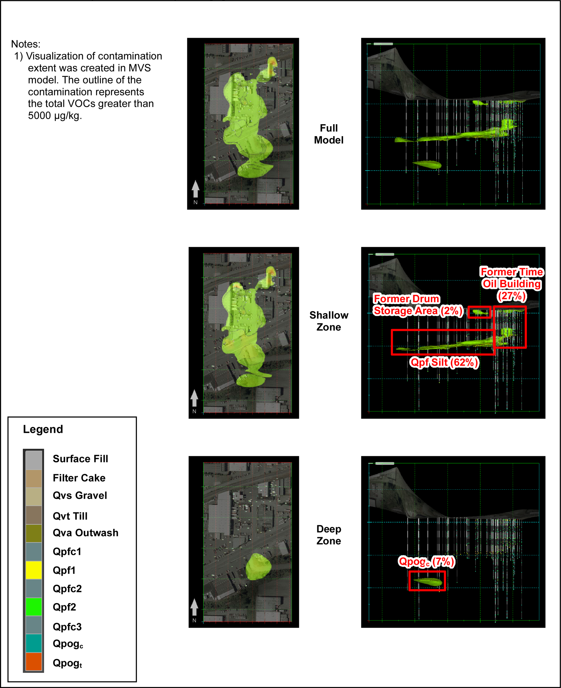
Figure B-9. 3D Visualization of the extent of soil contamination.

Source: Courtesy of CDM Smith.

Table B-6 provides the MVS™-modeled estimates of the contaminated volumes within different stratigraphic units and within different volumes across the Well 12A source area.

Nature and Extent of Contamination – Groundwater

Groundwater analytical data for the six primary COCs (PCA, PCE, TCE, cis-1,2-DCE, trans-1,2-DCE, and VC) were input into the existing 3D model. In general, the model includes the most recent groundwater VOC data for each well location from 2008 to the present. The model was used to visualize the contaminant plume distribution so the extent and mass of the COCs in groundwater could be evaluated. The groundwater plume domain was created using the rectilinear option, to size the domain to include all of the Time Oil source area wells and also nearby bounding wells (e.g., CBW-10 and CH2M-2). The groundwater domain was bounded on the bottom by the aquitard (Qpogt).

Figure B-10 shows the modeled extent of groundwater contamination where either TCE or cis-DCE exceeds 300 µg/L, 1,000 µg/L, and 3,000 µg/L. The 300 µg/L isopleth was used to illustrate the plume extent because it contains the known Time Oil source area and the majority of contaminant mass in groundwater. Therefore, it is referred to as the high concentration groundwater plume. Overall, the majority of the contaminant mass is distributed within the Qva, Qpfc, and Qpf units in the vicinity of the former Time Oil building with a deeper plume in the Qpogc unit extending across South Tacoma Way southwest of the Well 12A site. The high concentration groundwater plume is generally colocated with zones of elevated soil concentrations (sum of six primary COCs exceeding 5,000 µg/kg) generally associated with either the Qpf silt unit near the former Time Oil building or with the deeper Qpogc to the south of South Tacoma Way.

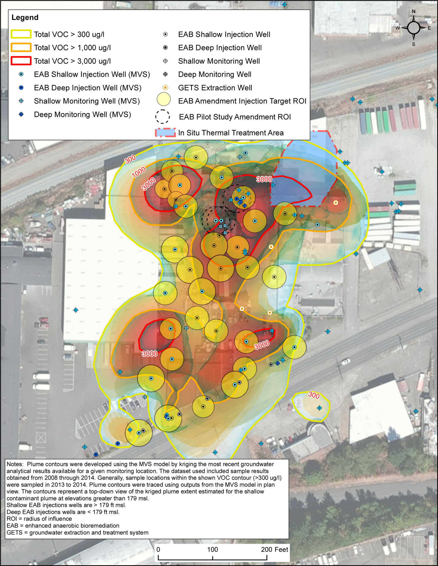
Figure B-10.Total VOCs in shallow groundwater (<179 ft) from 3D model 2014 upgrade.

Source: Courtesy of CDM Smith.

Mass Flux Transect

An evaluation of mass flux and mass discharge was conducted using a Theissen polygon method (ITRC 2010). This evaluation used groundwater samples collected from temporary monitoring points along a transect of the contaminant plume approximately perpendicular to groundwater flow. The vertical cross-sectional transect was divided into multiple discrete sub-areas of assumed uniform concentration and groundwater flow discharge (Nichols and Roth 2004). Mass discharge of groundwater was measured along the transect by combining the concentration and flow data (that is, Darcy velocity) to yield mass data in units of mass flowing normal to the control plane per unit of time. To characterize the Darcy velocity (q) across a plume transect, representative measurements are required for both the hydraulic flow gradient (i) and the hydraulic conductivity (K) of the flow system (where q = K * i).

For the mass flux calculations, the transect was divided into rectangles (polygons) that included depth intervals as follows:

• Vertical Interval 1: 40 ft–55 ft bgs for the Qva
• Vertical Interval 2: 55 ft–65 ft bgs for Qpfc1/Qpf, used when the Qpf unit is not present (the hydraulic conductivity of the Qpfc unit was used because it comprised a much greater percentage of the vertical area)
• Vertical Interval 3: 65 ft–75 ft bgs for Qpfc2
• Vertical Interval 4: 75 ft–95 ft bgs for Qpfc3
• Vertical Interval 5: 95 ft–115 ft bgs for Qpogc

Figure B-11 shows the results of the mass flux and discharge assessment for transect 1. Table B-7 presents the mass discharge measured for each stratigraphic unit for transect 1.

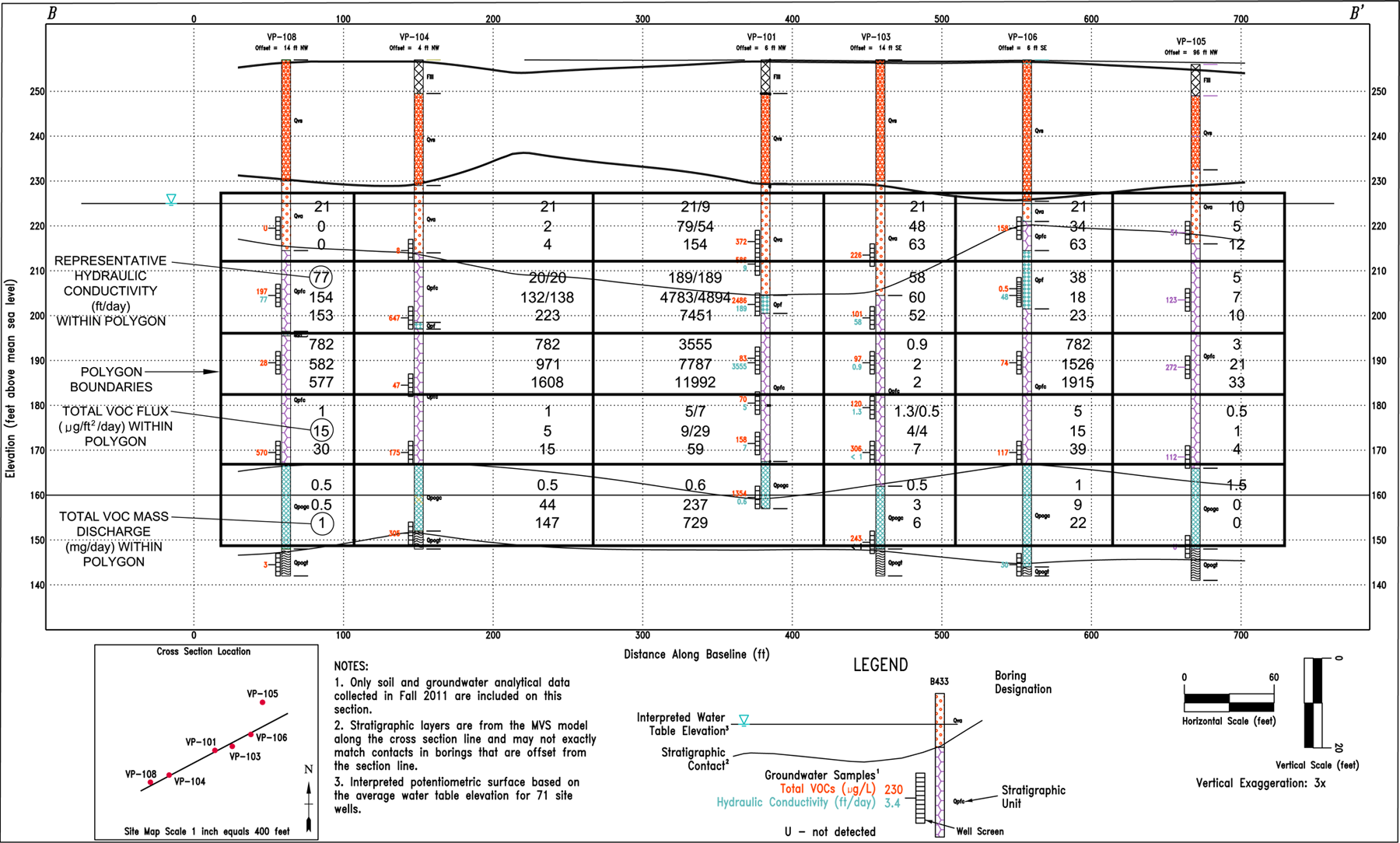
Figure B-11. Mass discharge-Transect 1.

Source: Courtesy of CDM Smith.

Results of the mass flux transect evaluation reveal that 96% of the total VOC mass discharge from Transect 1 came from intervals Qpfc1/Qpf and Qpfc2 (approximately 55 ft–70 ft bgs). In contrast, the Qva unit comprised only 1% of the measured discharge. In deeper intervals, the mass discharge declined with 1% accounted for in the Qpfc3 interval (75 ft–95 ft bgs) and 1% in the Qpogc interval (95 ft–115 ft bgs). In addition, nearly 78% of the mass discharge was associated with the central portion of the transect represented by VP101 (Figure B-10). A substantial proportion of the discharge consisted of degradation products cis- and trans-1,2-DCE, which totaled 40% of the mass discharge compared to 49% for TCE.

Mass Discharge Using GETS

Before the Well 12A source treatment technologies ISTR and EAB were implemented, the project team evaluated multiple methods for measuring contaminant mass discharge and selected one to assess compliance with the interim groundwater RAO (CDM Smith 2011, CDM Smith 2012b, CDM Smith 2013). Contaminant mass discharge measured with a pumping test using the GETS was selected as the compliance metric for the Well 12A site interim remedy. Subsequently, the baseline mass discharge using the GETS pumping test was 403 gallons per day (gpd) total VOC (TVOC) as the sum of PCA, PCE, TCE, DCE, trans-DCE, and VC and agreed to by the project team (CDM Smith 2013). The mass discharge baseline measurement of 403 gpd TVOC was calculated as the mean of three consecutive mass discharge measurements conducted approximately two weeks apart that met the following criteria:

• Extraction well rates were within 10% of target flow rates (defined as rates demonstrated to capture the target capture zone) during the mass discharge evaluation period.
• The TVOC concentrations (629, 613, and 592 μg/L) measured in samples collected from the influent sample port (SP)-1 of the treatment system) during each of the three mass discharge measurements had a relative percent difference of less than 18.5%, the practical analytical/sampling/operational variability for TVOC achievable based on historical SP-1 data (CDM Smith 2013).

The GETS pumping test will be used to assess if at least a 90% reduction in contaminant mass discharge is achieved following ISTR and EAB treatment within the Well 12A source area.

The mass discharge was measured using four extraction wells designed to capture and treat the contaminant plume from the source area. Figure B-9 shows the mass discharge measured at each of the extraction wells and the capture zone of each well using particle tracking modeling. The relative percentage of mass discharge from each of the extraction wells was also used to evaluate the strength of the source areas across the Well 12A source area to aid in selecting technologies, and to evaluate how treatment within different areas would affect contaminant mass discharge measured with the GETS.

Mapping Technologies - ISTR and EAB

The contaminant mass and extents, contaminated areas and volumes, and contaminant mass flux and discharge data were used to map treatment technologies (particularly ISTR and EAB) across the site to most efficiently address the contaminant mass and achieve the mass discharge reduction goal. Mapping technologies was focused on the following:

• maximizing the mass of contaminant removed and addressing mobile NAPL within the Time Oil building area
• maximizing the reduction of contaminant mass discharge while minimizing the footprint of aggressive/expensive technologies
• identifying the extent of the secondary source area where significant contaminant mass discharge is occurring outside the Time Oil building
• mapping EAB to areas that further contaminant mass discharge reduction, thereby achieving the reduction goal while minimizing the necessary treatment volume (in particular, the vertical extent)

To achieve these objectives, the following were evaluated: various treatment volumes, associated contaminant mass within the treatment volumes, and estimated contaminant mass discharge from the treatment volumes. Table B-8 summarizes the outcome of this volumetric contaminant mass and the volume estimates for the designated excavation, ISTR, and EAB treatment zones. The treatment technologies were mapped based on maximizing contaminant mass removal from the Time Oil building NAPL zone with aggressive technologies (excavation and ISTR) to address a significant proportion of the mass and a more significant proportion of the total contaminants discharged to the GETS.

ROD Amendment #2 identified ISTR as the selected remedy for the highly impacted portions of the deep vadose zone and upper saturated zone near the former Time Oil Building. The ISTR treatment zone presented in the FFS (CDM Smith 2009) was based on modeling of historical soil data collected between 1985 and 2004. The ISTR treatment zone finally selected was noticeably different from that presented in the FFS. With the addition of the pre-design investigation soil data, the modeled soil plume had shifted to the west such that the majority of the treatment area (approximately 76%) was located within the footprint of the former Time Oil building. The majority of the soil contaminant mass was found to be located in two distinct zones. The vadose zone and saturated zone beneath and in the vicinity of the former Time Oil building account for an additional 27% of the soil VOC mass >5,000 µg/kg. In general, the predesign investigation served to better bound the soil plume to the east and south and to confirm its presence beneath the Time Oil building, resulting in a significant reduction in uncertainty associated with the delineation.

The modeling performed to date suggests that, together, the EAB and ISTR treatment zones contain approximately 90% of the total VOC mass >5,000 µg/kg (see Figure B-9). While the Qpf silt unit contains approximately 63% of the contaminant mass in soil, it contributes approximately half the contaminant mass discharge from the site as measured using the GETS pumping evaluation. Likewise, the total contaminant mass near the Time Oil Building area is a much smaller area—13,000 square ft (sf) compared to 162,000sf—but contributes approximately the remaining half of the contaminant mass discharge to the GETS (measured by taking discharge to EW-5 plus half the discharge going to EW-3).

Therefore, ISTR treatment was mapped to the zone covering an area of approximately 13,000sf and extends from the ground surface (approximate elevation 254 ft amsl) to a depth of 55 ft bgs (elevation 199 ft amsl). This zone contains an estimated 27% of the VOC mass in soil and the majority of remaining mobile NAPL; for the reasons noted above, it is also believed to be responsible for approximately half of the contaminant mass discharge from the site. Approximately 74% of the treatment area is within the footprint of the former Time Oil building, with 30% beneath the older southern portion of the former Time Oil building. Although the ISTR treatment volume was similar to what had initially been conceptualized, the location of the area changed significantly with the majority of it being beneath the Time Oil building.

The EAB treatment zone was delineated to address additional isolated hotspots and the secondary source of contamination in the Qpf silty clay. This area is much larger (approximately 162,000 sf vs. 13,000 sf) compared to the ISTR treatment zone, and contains approximately 63% of the remaining mass responsible for approximately half of the mass discharge to the GETS. The mass flux evaluation with the transect evaluation demonstrated that an estimated 96% of the mass discharge in the high-concentration groundwater plume could be addressed by focusing treatment on the 10 ft–15 ft interval around the Qpf silt secondary source. Therefore, the vertical treatment interval for EAB (interval targeted for amendment injection) was refined from 50 ft to approximately 10 ft–15 ft. This provided substantial cost savings in reduced amendment volumes required for treatment.

Table B-9 summarizes the projected cost of the EAB remedy based on the actual implementation cost, but adjusted over the treatment volume (assuming the 50 ft treatment zone), compared to the approximate total final costs with revised treatment strategy (based on a more robust CSM informed by high-resolution characterization). In this case, the characterization did not result in a significant change in the target treatment area, but did result in a significant change in the vertical interval for treatment. Reducing the target vertical interval for treatment from 50 ft to 12 ft (average), with a deeper treatment zone with a 5 ft thickness in a smaller portion of the site, reduced the overall treatment volume by approximately 70%. This lowered the overall cost of the remediation by reducing costs for amendment, well installation, and labor for amendment injection for one full-scale injection event—from an estimated from $4.66 million to $1.66 million. The cost of the high-resolution characterization for the site was approximately $350,000. Even with this additional characterization cost, however, the project saved an estimated $2.65 million due to the substantial reduction in treatment volume.

Conclusions

High-resolution vertical profiling to evaluate contaminant distribution in heterogeneous media and assessing mass flux and mass discharge provided significant benefits to the project that aided in making key decisions and cost savings. Some key conclusions are as follows:

• Treatment technologies could be mapped effectively to address the contaminant mass discharge coming from the site.
• The primary NAPL source near the Time Oil building was relatively discrete in area and volume, but was responsible for nearly half the mass discharge coming into the GETS. Therefore, an aggressive (and expensive) treatment technology, ISTR, was mapped to this volume.
• The architecture of the contaminant mass of the Time Oil building source area was significantly different than that presented in the previous CSMs. Although the area of the ISTR treatment zone did not change significantly, the location changed dramatically.
• A significant secondary source area was determined to be associated with a discrete silty-clay layer present across a large area of the site. This area actually contained more contaminant mass in soil than the area near the Time Oil building, but was present in a very discrete interval of the aquifer, and discharge significantly less contaminant mass to the GETS. Therefore, EAB was mapped across a relatively large area, which was similar to that originally conceptualized; however, the vertical treatment interval was reduced from 50 ft to approximately 12 ft (with an additional 5 ft interval included in a deeper zone in a much smaller footprint of the area). This resulted in an approximately 70% reduction in the treatment volume.
• Innovative EAB amendments, using shear-thinning fluids, were designed and used for full-scale injections that allow fluids to be delivered more effectively in and around the Qpf silt layer.
• The pumping test method using the GETS was determine to be the best way to measure contaminant mass discharge reductions to achieve the compliance goal for the interim remedy.